Multi-class Classification of Mathematical-Numbers | CNN | Part4

25 min readNov 13, 2021

Below is the simple CNN based architecture, which we shall be building as part of this blog :-

A colourful representation of the CNN would look something like below :-

In case you are directly landing here, it’s highly recommended to have a view at this story.

In this blog, we shall be using KERAs framework with TensorFlow backend, in order to create a Convolutional Neural Network. We shall be using MNSIT dataset, which consists of 28*28 grayscale images, representing the hand-written images of numeric digits 0 to 9. The dataset is partitioned in 2 parts :-

Training dataset of 60,000 images.
Testing dataset of 10,000 images.

Question: What is the purpose of Convolutional-Neural-Networks ?

Question: What is the input given to Convolutional-Neural-Networks ?

Question: How does Convolutional-Neural-Networks works ?

Question: What are the other applications, where Convolutional-Neural-Networks can be used ?

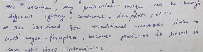
Question: Why is Image Classification that hard area of work ?

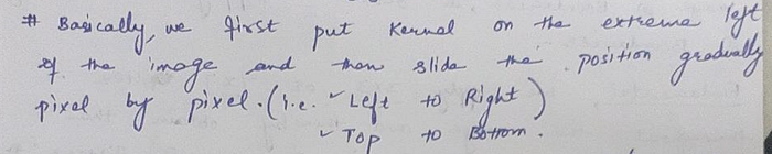
Question: How do we actually use “Convolution-Operation” in CNN to extract features ?

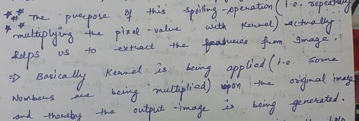
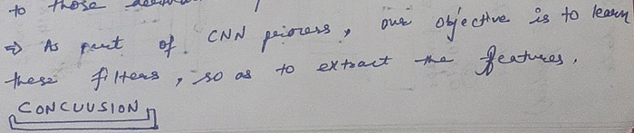
Question: What’s the purpose of performing Convolution-Operation (i.e. Applying Kernel(aka filter) on the input-image) ?

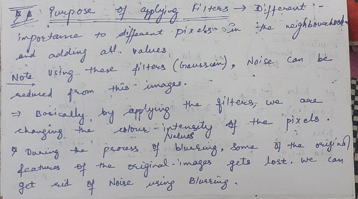
Question: Does Applying Kernel/Filters on the input-image NOT spoils the image pixels ? What advantage does it provides otherwise ?

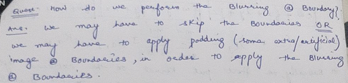
Question: How do we perform the blurring at the boundaries ?

Question: How does a simple 3*3 kernel(a.k.a. filter) looks like ?

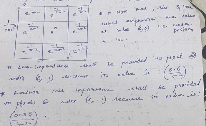
Question: Can a kernel be more complex as well ? Well, how does a Gaussian Filter looks like ?

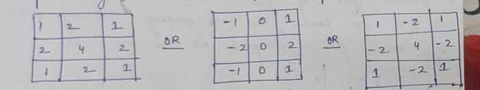
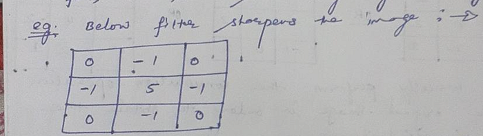
Question:- Are there some examples of filters (aka kernel) in order to sharpen the Image ?

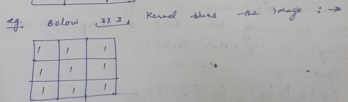
Question:- Are there some examples of filters (aka kernel) in order to blur the Image ?

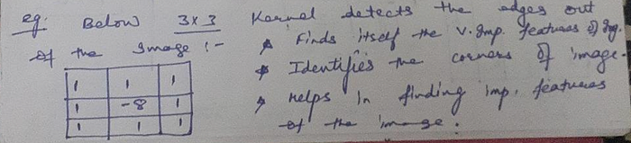
Question:- Are there some examples of filters (aka kernel) in order to detect the edges of the Image ?

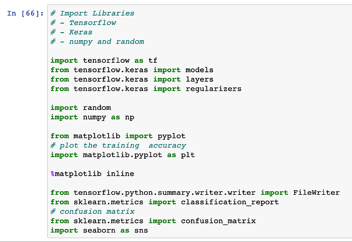
Let’s get back to our problem statement of multi-class-classification, where we would be classifying, the input image into 1 amongst 10 classes of decimal-digits (0 to 9). First, we import important libraries that we shall be using throughout our demonstration. We shall be using the tensorFlow V1 throughout the setup, therefore we explicitly also disable the TF V2 behaviour.

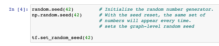
Next, we initialise the random-number-generator & set the seed so that, we can keep on using the same set of instances or random-numbers in every run of the program.

We would be using the MNIST hand-written data-set, which is already provided as a built-in data-set in the KERAs framework. We, therefore first create the instance of MNIST dataset and also divide the overall-dataset into Training & Testing parts.

Let’s first understand the meaning of the 4 variables created above :- The training set is a subset of the data set used to train a model.

Xtrain is the training data set.
Ytrain is the set of labels to all the data in Xtrain.

The test set is a subset of our data-set, that we shall be using to test our model, after the model has gone through initial vetting by the validation set.

Xtest is the test data set.
Ytest is the set of labels to all the data in Xtest.

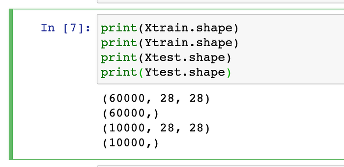
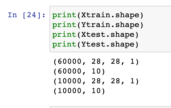
Coming back on the MNSIT dataset, let’s go ahead and print the shape of all of the above 4 datasets. We have following configuration :-

Training dataset of 60,000 images, stored in Xtrain.
Testing dataset of 10,000 images, stored in Xtest.

Also, please note that, this is set of hand-written numbers, stored as gray-scale-images. Each image is being stored as the matrix of size, 28 * 28 with pixel values taking a value from in range (0 to 255).

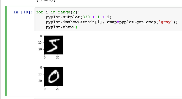
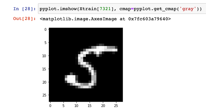
Let’s go ahead and visually see some of the images in our training data-set :-

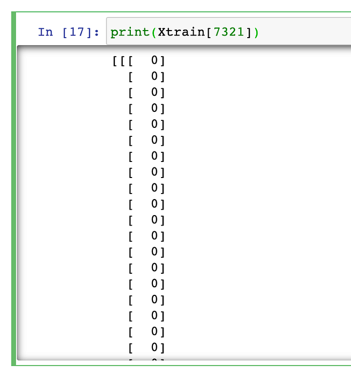
Let’s see the shape of any random image(say we wanna investigate 7321th image) from the training dataset and also view the pixel-values of this random image :-

Data Pre-Processing Operation :- Here, we shall be performing 2 operations namely, on the entire dataset (i.e. Training + Test data-set) :-

Reshaping.
Normalisation.

Step #1.) Note that, each gray-scale image usually has depth value of 1, therefore let’s perform the reshape() operation here on the entire training dataset :-

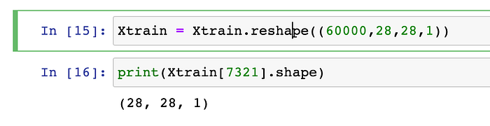
Step #2.) Now, let’s view the pixel-values of this random image again now. Note that, the image has now changed to 3d image.

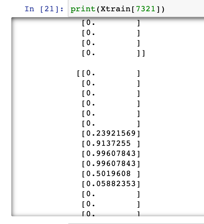
Step #3.) Now, let’s perform the Normalisation operation at this random image. Note that, shape would not change, post normalisation operation :-

Step #4.) Again, let’s re-observe the pixel-values of this random image now. Note that, pixel-values have duly changed to decimal values now :-

Step #5.) Observe that, even after reshaping+normalisation operations here, we can still visually see any image. Let’s go ahead and see our own random image i.e. 7321th imae :-

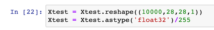
Step #6.) Let’s also perform the same aforesaid operations on the test dataset too :-

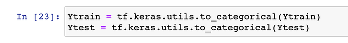
Step #7.) Next, note that, the output values into the data-set are categorical in nature with values in range of (0 to 9). Therefore, this categorical data is first converted into vector using One-Hot-Encoding approach. Keras library provides us out-of-the-box method to “to_categorical”.

Step #8.) Now, let’s view the value being stored in output(Ytrain) for this random image again now. Note that, since the 7321th image was

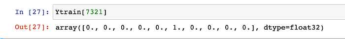
Step #9.) At-last, here is our total dataset looks like :-

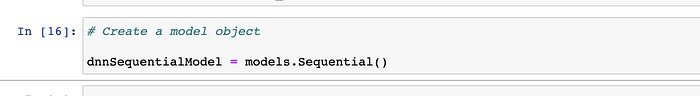
Let’s now build the simplest & sequential DNN using Keras. We are planning to use the 4 layers in this Neural Network.

Step#1.) First Layer is a Conv2D layer, which is defined as a follows :- This is a Conv2D layer of 32 Kernels(aka filters) each of size 3 * 3 and RELU activation-function.

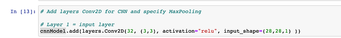
Conv2D is a layer which performs 2D convolutions, with filter of size 3*3. There are 32 such filters (aka kernels), that we have specified in the initial go here. Here, In this convolutional-operation, stride-size of 1 is being considered. All of these 32 filters are initialised randomly by it’s own.
The input_shape represents the size of the input-image to this CNN model. Each image is having dimension (28 * 28) with depth of 1.

Question:- How does a simple convolutional i.e. Cross-CoRelation (Operation of applying Filter/Kernel over the Input Image) operation looks like ?

Question:- How is the above filter(kernel) actually applied on the input-image ?

Question:- What’s the objective of a CNN model ?

Question:- How does the architecture looks like for the first layer of this CNN ?

Note: It basically means that, on each of the Input-Image from the training data-set, we are applying the 32 different filters(aka kernels) and therefore, for each input-image, there shall be 32 feature-Maps shall be generated.

Question:- What does each convolutional-plane in above architecture represents ?

Question:- Since our original-input-image was of dimension (28*28*1), why is that size of the each of the output-feature-map shrinks to (26*26*1) ?

Note: The size of the output-feature-map is governed by the below formula basically. It depends upon following factors :-

Input-size of Image.
Kernel-size.
Stride-size.
Padding-size.

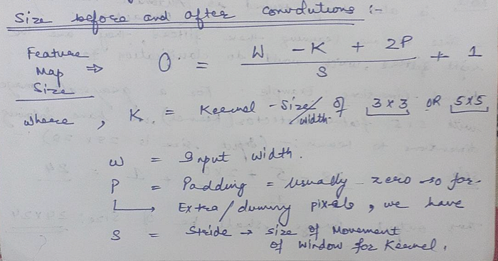
In our case, we have : W=28, K=3, P=0, S=1, therefore, computation for Output-Feature-Map-Size shall be :- O = [(28–3 + 2*0)/1 + 1] = 26.

Question:- What would be immediate impact, if we have Stride-value as more than 1 ?

Question:- Can we visualise, how does our output-feature-maps looks like, post this first-layer’s convolutional operations being applied ?

Note: As we explained above :-

Each of 32 output-feature-maps would be of size (26*26) with depth as 1.
There are 32 output-feature-maps, because we took 32 filters initially for Layer-1.

Question:- Can we know, the computation behind 320 trainable parameters in Layer 1 ?

See here we have a single-input-image (with 1 feature maps aka 1 dimensions aka 1 depth) as Input to the 1st Convolutional layer.
There are 32 kernels, each of size : 3*3. Note that, In each of the filter, we have got 9 different values. So, total no. of parameters comes out to be :~: (1 * 32 * 9) = 288.
Also, there is A bias, each one for each of the 32 filters. So, there are 32 biases.
Hence, total number of parameters comes to be:- 288 + 32 == 320.

Step#2.) Layer-1’s MaxPooling operation downsamples the feature-map, by taking the max out of the window. Here in above example, stride of 2*2 is being added, which indicates that, pooling-window moves with this speed.

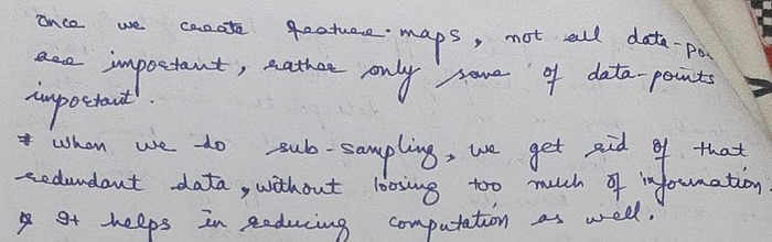
Question:- What’s the importance/objective of applying Sub-Sampling-Operation (aka Pooling) ?

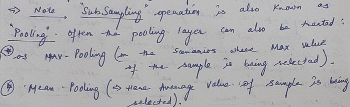
Question:- What are the various types of the Sub-Sampling (a.k.a. Pooling) Operations available ?

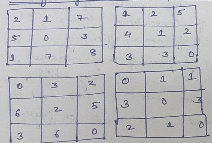
Question:- Consider an example of Max-Pooling-Operations : Given an below output-feature-maps of size (6*6), what shall be output of :-

Max-Pooling-Operation.
Mean-Pooling-Operation.

The output of Max-Pooling-Operation would look something like below :-

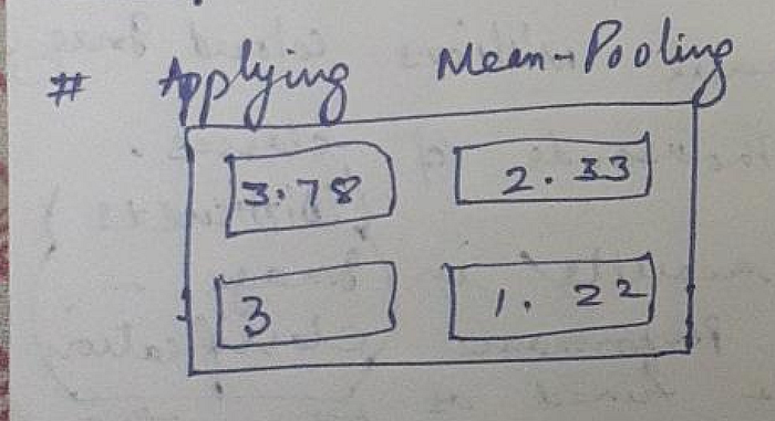
The output of Mean-Pooling-Operation would look something like below :-

Question:- Can we visualise, how does our output-feature-maps now looks like, post this first-layer’s Max-Pooling-Operation being applied ?

Note: The size of the output-feature-map is now reduced to (13*13), because of 2*2 pooling being applied over the same

Step 3#.) Coming back to the Second Layer which is again an another Conv2D layer, which is defined as a follows :- This is a Conv2D layer of 64 Kernels(aka filters) each of size 3 * 3 and RELU activation-function.

Conv2D is a layer which performs 2D convolutions, with filter of size 3*3. There are 64 such filters (aka kernels), that we have specified in this layer here. So, for each Incoming-Input-Feature-Map, there shall be 64 outputs thus generated, as a result of application of each of 64 kernels.
Note that, input size to the Layer-2 is (13*13*1) and therefore, the size of the output-feature-map of this 2nd layer shall be dictated by following computation :- We have : W=13, K=3, P=0, S=1, therefore, computation for Output-Feature-Map-Size shall be :- O = [(13–3 + 2*0)/1 + 1] = 11. Therefore, each of the 64 output-feature-maps this generated post this convolution-operation of 2nd Conv-Layer shall be (11*11*1).

Question:- Can we visualise, how does our output-feature-maps looks like, post this 2nd-layer’s convolutional operations being applied ?

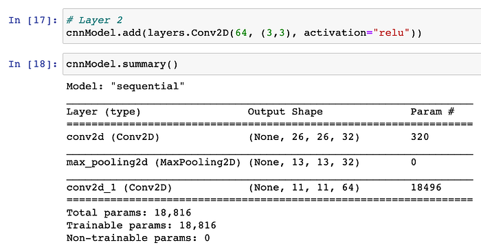
Question:- Can we know, the computation behind 18,496 trainable parameters in Layer 2?

See here we have a single-input-image (with 32 feature maps aka 32 dimensions) as Input to the 2nd Convolutional layer.
There are 64 kernels, each of size : 3*3. Note that, In each of the filter, we have got 9 different values. So, total no. of parameters comes out to be :~: (32 * 64 * 9) = 18,432.
Also, there is A bias, each one for each of the filter. So, there are 64 biases.
Hence, total number of parameters comes to be:- 18,432 + 64 == 18496.

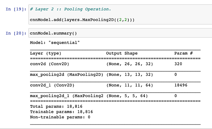
Step#4.) Layer-2’s MaxPooling operation downsamples the feature-map, by taking the max out of the window. Here in above example, stride of 2*2 is being added, which indicates that, max-pooling-window moves with this speed.

Question:- Can we visualise, how does our output-feature-maps’s size now looks like, post this second-layer’s Max-Pooling-Operation being applied ?

Step 5#.) Coming back to the Third Layer which is again an another Conv2D layer, which is defined as a follows :- This is a Conv2D layer of 64 Kernels(aka filters) each of size 3 * 3 and RELU activation-function.

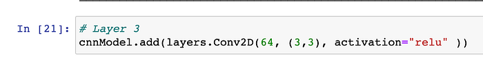
Conv2D is a layer which performs 2D convolutions, with filter of size 3*3. There are again 64 such new filters (aka kernels), that we have specified in this layer too. So, for each Incoming-Input-Feature-Map, there shall be 64 outputs thus generated, as a result of application of each of 64 kernels.
Note that, input size to the Layer-3 is (5*5*1) and therefore, the size of the output-feature-map of this 3rd layer shall be dictated by following computation :- We have : W=5, K=3, P=0, S=1, therefore, computation for Output-Feature-Map-Size shall be :- O = [(5–3 + 2*0)/1 + 1] = 3. Therefore, each of the 64 output-feature-maps this generated post this convolution-operation of 3rd Conv-Layer shall be (3*3*1).

Question:- Can we visualise, how does our output-feature-maps looks like, post this 3rd-layer’s convolutional operations being applied ?

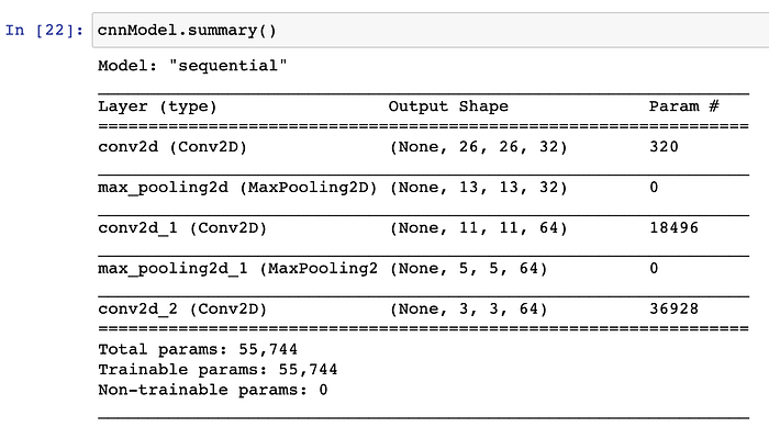
Question:- Can we know, the computation behind 36,928 trainable parameters post Layer-3’s convolutional operation ?

See here we have a single-input-image (with 64 feature maps aka 64 dimensions) as Input to the 3rd Convolutional layer.
There are 64 kernels, each of size : 3*3. Note that, In each of the filter, we have got 9 different values. So, total no. of parameters comes out to be :~: (64 * 64 * 9) = 36,864.
Also, there is A bias, each one for each of the filter. So, there are 64 biases.
Hence, total number of parameters comes to be:- 36,864 + 64 == 36,928.

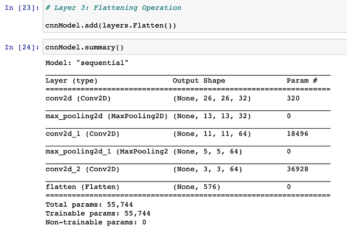
Step#6.) Layer-2’s Flattening Operation : Keras Flatten() class is very important when we have to deal with multi-dimensional inputs such as image datasets. Keras.layers.Flatten() function flattens the multi-dimensional input tensors into a single dimension, so we can model our input layer and build our neural network model, then pass those data into every single neuron of the model effectively.

Step 7#.) Coming back to the Fourth Layer which is a Dense-Layer with 64 neurons and RELU activation-function.

This layer also acts as an input layer, with input-tensor of size: (576*1) i.e. each input image to our fully-connected-model is of size 576*1.
Recall that, earlier above, we had converted(reshaped/flattened) all of our input images from 3d (dimension: 3*3*64) to 1d (dimension: 576).
This 4th layer is defined as dense-layer with 64 neurons and ‘relu’ activation function.
Dense-Layer implies that, all neurons of one layer are connected to all neurons of next layer.
There would be 64 outputs, from this 4th Layer, because there are 64 neurons overall we have in this particular 4th layer. Below is the summary, post applying this layer to our model :-

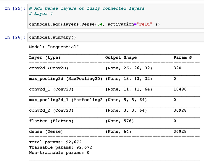
Computation of no. of variables involved in First hidden layer (aka 4th layer of the CNN model) :-

Input to the first hidden layer(aka 4th layer of CNN) is an flattened feature-map of size (576*1).
In first hidden layer, we have in-total of 64 neurons, so, the total number of variables involved are :- 576*1*64 = 36,864.
Also, there would be 64 total biases each-one for 64 neurons there in first hidden layer(aka 4th layer of CNN). Therefore, here in this model, total net number of parameters would be : (36,864 + 64 == 36928).

Step 8#.) Coming back to the Fifth Layer (aka 2nd hidden layer) which is again a Dense-Layer having 32 neurons and RELU activation-function.

This layer also acts as a hidden layer, with input-tensor of size: (64*1). Recall that, output of the first hidden layer was an image of size 64*1.
This 5th layer is defined as dense-layer with 32 neurons and ‘relu’ activation function. Dense-Layer implies that, all neurons of one layer are connected to all neurons of next layer.
There would be 32 outputs, from this 5th Layer, because there are 32 neurons overall we have in this particular 5th layer. Below is the summary, post applying this layer to our model :-

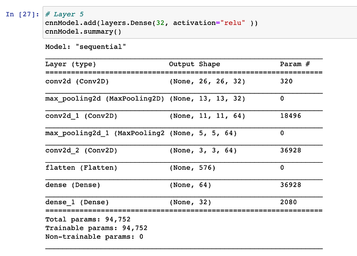
Computation of no. of variables involved in Second hidden layer (aka 5th layer of the CNN model) :-

Input to the second hidden layer(aka 5th layer of CNN) is a flattened feature-map of size (64*1).
In second hidden layer(aka 5th layer of CNN model), we have in-total of 32 neurons, so, the total number of variables involved are :- 64*32 = 2048.
Also, there would be 32 total biases each-one for 32 neurons there in second hidden layer(aka 5th layer of CNN). Therefore, here in this model, total net number of parameters would be : (2048 + 32 == 2080).

Step 9#.) Coming back to the Sixth Layer which is also an output Layer with 10 neurons and SOFTMAX activation-function.

This layer also acts as an output layer, with input-tensor of size: (32*1). Recall that, output of the second hidden layer was an image of size 32*1.
This 6th layer is defined as dense-layer with 10 neurons and ‘softmax’ activation function.
There would be 10 outputs, from this 6th Layer, because there are 10 neurons overall we have in this particular 6th layer.
Note that, we have used softmax activation function, in order to perform the Classification accurately. Below is the summary, post applying this 6th layer to our model :-

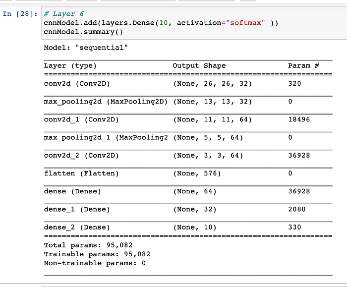
Computation of no. of variables involved in Output layer (aka 6th layer of the CNN model) :-

Input to the 6th layer of CNN is a flattened feature-map of size (32*1).
In 6th layer(aka final output layer of CNN model), we have in-total of 10 neurons, so the total number of variables involved are :- 32*10 = 320.
Also, there would be 10 total biases each-one for 10 neurons there in output layer(aka 6th layer of CNN). Therefore, here in this model, total net number of parameters would be : (320 + 10 == 330).

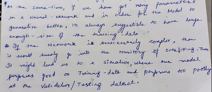
Note that, we have in-total of 95,082 parameters involved in this 6-layered-CNN model. In order to generalise the model better, it’s always suggestible to have large size of the training-data-set.

Finally, our Six-Layered-CNN-model, thus formed so far, can also be visualised as below :-

Step 10#.) Configuring Model :- Let’s now configure our recently created DNN model for training.

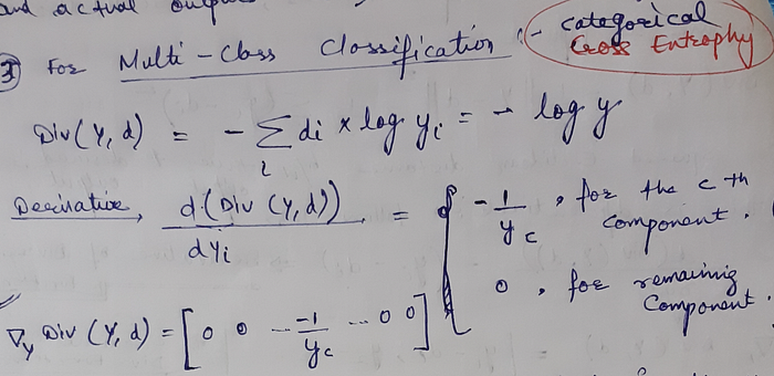
The Cost function is defined as Loss-Function and in this case, we are using “Categorical-Entropy” as Loss function.

The metrics used for evaluating the model is “accuracy”.
We are planning to use ADAM optimiser on the top of SGD (Standard Gradient Descent), in order to minimise the cost-function.

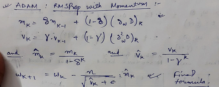
Usually, below values are adopted for hyper-parameters Delta and Gamma :-

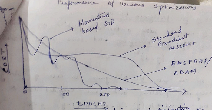
Here is a ready comparative analysis for various types of Optimisers :-

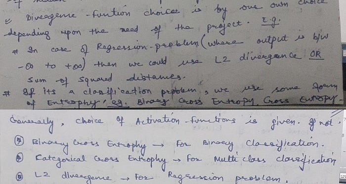
Question: What should be our choice of selecting a Cost/Loss/Divergence Functions ?

Once the configuration of our model is complete, we can proceed for Training.

Step 11#.) Training of Model :- Given the enormous(60K) data-set that we have got, we shall not be using “Full-Batch-Gradient-Descent” because of expensive computation being involved there, therefore we are planning to use “Mini-Batch-Gradient-Descent” approach, in order to minimise the LOSS.

Let’s understand few things from above step :-

Epoch :- One Epoch is when an ENTIRE dataset is passed forward and backward through the neural network only ONCE. We usually need many epochs, in order to arrive at an optimal learning curve. Here, in this example, In one Full-Epoch (i.e. Forward+Backward pass), these 938 batches are passed. Weights are iteratively tuned, Loss is gradually reduced and Model-accuracy is gradually improved.

Question:- Why do we need more number of EPOCHS ?

One epoch is not enough, as it may lead to under-fitting of the curve. As the number of epochs increases, more number of times the weight are changed in the entire neural network and the curve usually goes from under-fitting to optimal to over-fitting curve.

Batch size: Since we have limited memory, probably we shall not be able to process the entire training instances(i.e. 60,000 instances) all at one forward pass. So, what is commonly done is splitting up training instances into subsets (i.e., batches), performing one pass over the selected subset (i.e., batch), and then optimising the network through back-propagation. So we have divided our Training-Data-Set into the small chunks of 64 each. Therefore, there are around 60,000 / 64 ~==~ 938 net-total batches that we have formed in this process.

Question: What’s suggestible regarding Batch-Size ?

The higher the batch size, the more memory space we would be needing. The batch_size is usually specified in power of 2.

Example #1: Let’s say we have 2000 training examples that we are going to use, then we can divide the dataset of 2000 example-instances into batches of 500, then it will take 4 iterations to complete 1 complete epoch.

Example #2: Coming back to our above example, we have 60,000 training examples, and our batch size is 64, therefore, it will take us 938 iterations to complete 1 epoch. Note that, in each epoch → all 60,000 instances shall be processed for sure. Also observe that, after every epoch, the loss reduces and accuracy improves.

Validation Split of 0.1: It means that out of total dataset, 1% of data is set aside as the cross-validation-set. It’s value is a Float between 0 and 1. It stands for the fraction of the training data to be used as validation data. The model will set apart this fraction of the training data, will not train on it, and will evaluate the loss and any model metrics on this data at the end of each epoch.

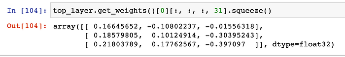
Question:- So, we know that Layer-1st had got 32 filters/kernels overall and during the course of training our model, basically our goal was to learn these kernels itself. Post the training process, can we know, what weights had been learnt by our CNN model for 31st kernel of Layer-1st ?

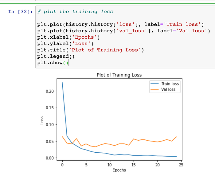
Question: Can we visualise the Validation-Loss, as the various epoch progresses ? Yes, we can also plot the graph for Validation-Loss. Below graph signifies that :

As the no. of epochs progresses, validation-loss-value also decreases. Note that :-

Post 1st EPOCH is completed, net validation loss of our model was 6.34%.
Post 2nd EPOCH is completed, net validation loss of our model has reduced to 4.37%. This is a considerable improvement.
Post 3rd EPOCH is completed, net validation loss of our model has further reduced to 4.13%. This is further respectable improvement.

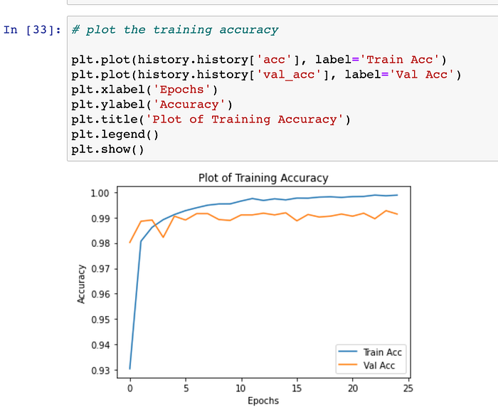
Step 13#.) Question: Can we visualise the Validation-Accuracy, as the various epoch progresses ? Yes, We can also plot the graph for Validation-Accuracy. Below graph signifies that : As the no. of epochs progresses, validation-accuracy also increases. Note that :-

Post 1st EPOCH is completed, net total accuracy of our model was 98.02%.
Post 2nd EPOCH is completed, net total accuracy of our model increased to 98.85%.
Post 3rd EPOCH is completed, net total accuracy of our model increased to 98.90%.

Step 14#.) As training of the CNN model progresses, both the (accuracy and loss) are stored as a list in the object. Final (Training Loss and Accuracy) can be obtained from the history object.

The last element of the history object (model_fit.history[‘loss’])gives us the final loss after training process.
The last element of the history object (model_fit.history[‘acc’])gives us the final accuracy after training process.

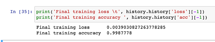
From above snapshot, we can observe that, our vanilla CNN model, is giving the training accuracy of 99.87% and overall testing loss is : .0039.

Step 15#.) Recall that, in the beginning, we had divided the entire MNSIT data-set into Training and Testing datasets. We had 10K records into out Testing-Dataset. Can we see the same please ?

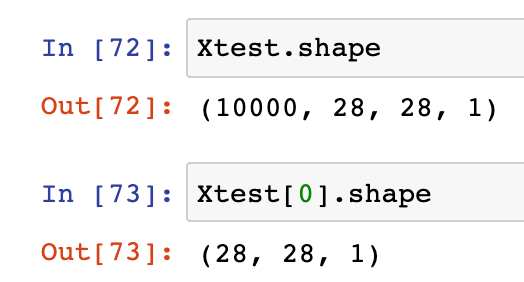
Above output indicates that, Xtest is the testing-dataset have got the 10,000 images and each image is of dimension 28*28 with depth as 1.

Step 16#.) Can we see any sample random image from the testing dataset(Xtest) and it’s corresponding label in the test-dataset(Ytest) ?

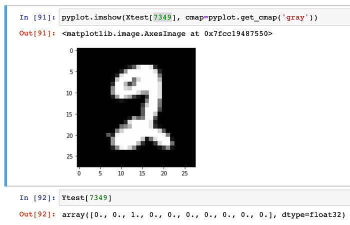
Note that, earlier above, we had converted the Ytest as well into the vector representation, using the one-hot-encoding approach. Therefore, the corresponding label for the sample random image appears into the vector-format-representation.
In the one-Hot-encoding-format, each position represents the number. For example, Index-0 represents 0. Index-1 represents 1, Index-2 represents 2. and so on.
Note that in above example, we have randomly chosen the 7349th image from the testing-data-set and same upon being converted to the one-hot-vector format, indicates that position 3rd from beginning is ONE and rest other are ZERO)

Step 17#.) As our CNN model is all ready now, let’s proceed to perform our long-desired task of prediction of the numbers ?

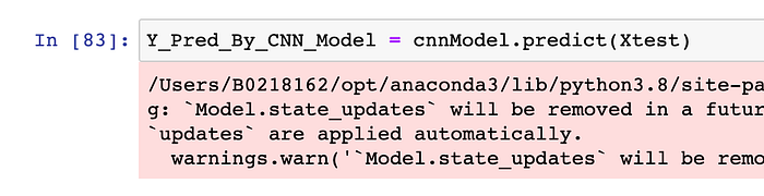
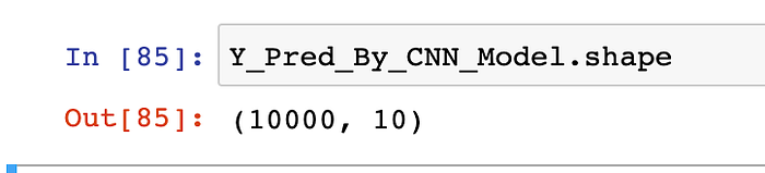
Question:- We had 10K images into our testing-data-set. Are you sure that, we have got the prediction being done for all 10K images ?

Question:- Can you show us for example, what result is being predicted by our respected-CNN model, for the same random image i.e. 7349th image, for which we above saw the actual-results ?

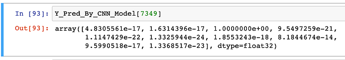
Note that, this is again a vector-formatted-result and the value at 2nd index is too high whereas the values at all other 9 indices is too small.

High value @ 3rd Index, indicates that, our model is too much confident about this particular number being as 2.
Small value @ all other indices, indicates that, our model is too less confident about this particular number either being as 0 OR being as 1 OR being as 3 OR being as 3 OR being as 4 OR being as 5 OR being as 6 OR being as 7 OR being as 8 OR being as 9.

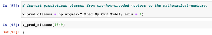
Step 18#.) This one-hot-encoded vector is getting difficult for me to visualise. Can you kindly convert this to plain-old mathematical numbers, back AND also show the result being predicted by our respected-CNN model, for the same random image i.e. 7349th image ?

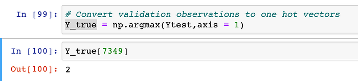
Step 19#.) Output of Step-18 looks so cool, Alright, let’s convert our entire Ytest dataset to plain-old mathematical numbers, back AND also show the actual-class for the same random image i.e. 7349th image ?

Step 20#.) Alright we were originally doing the Multi-Class-Classification of mathematical numbers. As we now have both the actual & predicted classes for YTest, can we visualise the classification-report please ?

Question:- For Number 7, what does precision of 0.98 indicates ?

Precision → Precision is the ratio of correctly predicted positive observations to the total predicted positive observations. The question that this metric answer is of all numbers that labeled as 7, how many actually got predicted as 7 ? High precision relates to the low false positive rate. We have got 0.98 precision which is pretty good. Precision = TP/TP+FP. In other words :-

When our model predicts that any number is 7, it is correct around 98% of the time.

Question:- For Number 8, what does recall of 0.98 indicates ?

Recall → The recall is the ratio TP / (TP + FN) where tp is the number of true positives and fn the number of false negatives. The recall is intuitively the ability of the classifier to find all the positive samples. In other words :-

For all the numbers 8 in our Test-Set, recall tells us, how many we correctly identified as 8.

F1-score → F1-score gives us the harmonic mean of precision and recall. The scores corresponding to every class will tell us the accuracy of the classifier-model in classifying the data points in that particular class compared to all other classes.

Support → Support is the number of actual occurrences of the class in the specified dataset. Imbalanced support in the training data may indicate structural weaknesses in the reported scores of the classifier and could indicate the need for stratified sampling or rebalancing. Support doesn’t change between models but instead diagnoses the evaluation process.

Step 21#.) Can we kindly visualise the Confusion-Matrix for this Multi-Class-Classification please ?

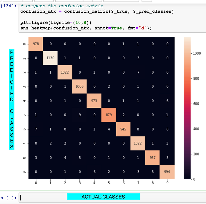
A Confusion matrix is an N x N matrix used for evaluating the performance of a classification model, where N is the number of target classes. The matrix compares the actual target values with those predicted by the machine learning model. This gives us a holistic view of how well our classification model is performing and what kinds of errors it is making.

Step 22#.) Next, We can evaluate our thus build model with the help of testing dataset of size 10,000. The “evaluate” function gives us the testing accuracy and testing loss as the output.

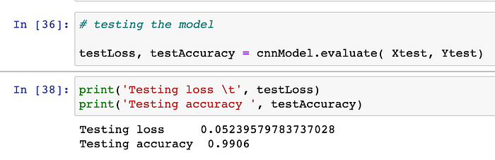
From above snapshot, we can observe that, our vanilla CNN model, is giving the testing accuracy of 99.06% and overall testing loss is : .052.

e can try to improvise this accuracy by playing on following parameters :-

By changing the number of Kernels being applied in the initial layers.
By changing the size of each kernel being applied on the input image.
By changing the type of sub-sampling-operation like MaxPooling OR MeanPooling.
By changing the number of neurons in each of the hidden/output layers.
By modifying the various optimisers like RMSProp, ADAM, etc.
Changing the number of hidden layers itself. (Note that, we have used 3 CNN layers and 3 hidden layers, in total, in aforesaid demonstration).
Changing the number of neurons in each of the involved layers (input/dense layer).
By playing on the value of the eTa i.e. Learning-Rate.
Choice of Activation functions at each layer.
By modifying the various optimisers like RMSProp, etc.
By testing out the CIFAR dataset.
By training for more epochs for better graphs.

Question:- Having understood all of the concepts above, what’s the ultimate requirement for being succesfull in getting good outputs from CNN ?

Thanks for reading through this and we shall meet you in another article.

References:-

Multi-class Classification of Mathematical-Numbers | CNN | Part4

Written by aditya goel